Understanding Impact of Traffic Congestion on Mobility and Cost from Large-Scale Taxi Trip Data

Data Description

The DC Taxicab trip data contains the taxi trips for either pick up or drop off locations within District of Columbia (DC), which can be downloaded from Open Data DC. The data is provided by the Department of For-Hire Vehicles (DFHV) of DC, and does not include car-sharing vehicles such as Lyft or Uber. The information of each trip can be represented with a tuple $<l_o, l_d, t_o, t_{od}, d_{od}, c_{od}>$ , where $l_o$ and $l_d$ are respectively the pickup and dropoff locations, $t_o$ and $t_{od}$ are respectively the pickup time (rounded to the nearest hour) and the whole trip time (in minutes), $d_{od}$ and $c_{od}$ are respectively the trip distance (in miles) and the total trip cost (in $) including meter fare, tip, surcharge, tolls, and extras. There are no vehicle identifiers in the data set. We consider the data in a one-year period between [2015-09-01, 2016-08-31] for this study, which includes totally 14.34 million Taxicab trips.

Basic Trip Characteristics

We study basic characteristics of taxi trips by exploring their temporal and spatial distributions and by analyzing their probability distributions as functions of the key trip attributes such as trip distance, trip time, and trip cost.

Fig. 1a shows hourly taxi trip rates of both weekday (in blue) and weekend (in red), where each trip rate is computed with the number of trips averaged by its number of associated days. For weekday, although high taxi trip rate occurs during common working hours and the high rate continues even for a few after-work hours, no obvious AM or PM peak is expressed in the hour-of-day distribution of taxi trip rates, which indicates that commuting may not be the primary function of taxi trips. For weekend, a high value of taxi trip rate is shown during midnight. This is consistent with our common sense that taxi trip may play a significant role for night life of weekend. Fig. 1b gives the comparison of hourly taxi trip rates among different seasons, which clearly shows some seasonal variations in the taxi trip rates.

Fig. 1c gives the spatial distribution of taxi trip rates by pickup locations, where pickup locations are decomposed with $k$ -digit grids using $k=3$ . In Fig. 1c, each circle represents the center of a pickup location decomposed with $3$ -digit grid, and its color represents the range of averaged daily taxi trip rate (i.e. averaged daily number of taxi trips) in $\operatorname{log}_{10}$ corresponding to the pickup location. As shown in the figure, the difference in the values of averaged daily taxi trip rate could reach even several orders of magnitude among different pickup locations. Fig. 1d shows the spatial distribution of the top 1000 highest O-D pairs in the ranking of taxi trip rates, where all O-D locations are decomposed with $k$ -digit grids using $k=2$ . In Fig. 1d, each line represents an O-D pair, and its color represents the range of averaged daily taxi trip rate in $\operatorname{log}_{10}$ corresponding to the O-D pair. As shown in the figure, the top 1000 highest O-D pairs ranking in taxi trip rates are clustered around the central business district of DC.

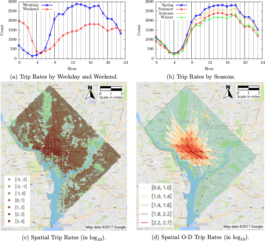
Figure 1: Temporal and Spatial Distributions of Taxi Pickup Trips.

Fig. 2 shows the empirical Probability Density Functions (PDFs) and Cumulative Distribution Functions (CDFs) of distance, time, and cost of taxi trips. In the statistical analysis, we exclude the outliers with $t_{od}\le 0$ , $d_{od}\le 0$ and $c_{od}\le 0$ .
We find that each of the three empirical PDFs can be well fitted with a lognormal distribution as shown below,

(1) $\begin{equation*} F(x | \mu, \sigma)=(x\sigma\sqrt{2\pi})^{-1}\operatorname{exp}({-\frac{\left(\ln x-\mu\right)^2}{2\sigma^2}}), \end{equation*}$

where $x$ is a key trip attribute such as trip distance, time, and cost, and the parameters $\mu$ and $\sigma$ are estimated using a global optimization algorithm \citep{xie2014cooperative} minimizing the least squares between the data and the fitting function. For the three empirical PDFs, the parameters ( $\mu$ , $\sigma$ ) are respectively (0.7623, 0.9223), (2.4555, 0.6004), and (2.4326, 0.4564), and the root-mean-square errors (RMSE) are respectively 1.51E-3, 6.75E-4, and 1.54E-3. The trip distance distribution gives the median and the 90th percentile of taxi trip distance as 1.68 and 5.72 miles, respectively. The trip time distribution gives the median and the 90th percentile of taxi trip time as 10.96 and 23.40 minutes, respectively. The trip fare distribution gives the median and the 90th percentile of taxi trip cost as $11.01 and $22.85, respectively.

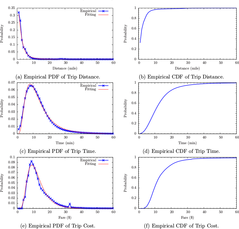
Figure 2: Statistics of Distance, Time, and Cost of Taxi Trips.

The two-parameter models on trip distance and time that are extracted from the taxi data in the DC area are consistent and complementary with the other recent works of the taxi data analysis in a few different cities, e.g., New York City. From the viewpoint of multimodal trip planning, the information of trip distance, time and cost is crucial for road users to make choice decision on transportation modes and travel routes. The two-parameter model is also useful for simulation studies on providing inputs. In addition, the model can be used for delivering a robust estimate of the mean value as $\operatorname{exp}(\mu+0.5 \cdot \sigma^2)$ in case that there exist significant outliers in data.

Mobility and Cost: Effect of Traffic Congestion

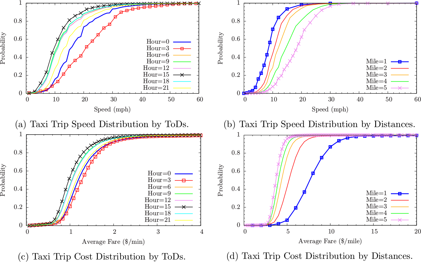
Mobility and cost are two key factors to consider as people plan their travels. Fig. 3 shows the comparisons of empirical CDFs of taxi trip speed (in mph) and cost (in $/min and $/mile) among different Times of Day (ToDs) and among different distances respectively, where the CDFs by ToDs are averaged over every three hours of day, and the CDFs by distance are averaged over every mile within five miles. For each panel of Fig. 3, we apply two-sample Kolmogorov-Smirnov tests on each pair of empirical CDFs to check if their difference in distributions is statistically significant. All the test results show that $p$ -values approach to $0$ , turning out that in each panel of Fig. 3, any two CDFs are different in statistical significance.

Figure 3: Distributions of Speed and Cost of Taxi Trips by ToDs and Distances.

For each taxi trip $i$ , the average speed is calculated as $v_{od}^{i}=d_{od}^{i}/t_{od}^{i}$ . Fig. 3a shows the empirical CDFs of taxi trip speed at different ToDs. During 3-6 AM, the taxi trip speed is the highest, where the median and 90th percentile of speed are 18.16 and 32.01 mph, respectively (see the rightmost curve in Fig. 3a). During 15-18 PM, the taxi trip speed is the lowest, where the median and 90th percentile of speed are 9.94 and 19.71 mph, respectively (see the leftmost curve in Fig. 3a).

Taxicabs can be seen as “floating cars” in urban traffic flows. Thus, speed of taxi trips can vary largely between different ToDs due to distinct urban congestion situations in traffic network. For measuring the impact of urban congestion, the {\em taxi-based congestion index} (TCI) is defined as

(2) $\begin{equation*} \text{TCI}=\tilde{V}_{\text{ToD}}^{max}/\tilde{V}_{\text{ToD}}, \end{equation*}$

where $\tilde{V}_{\text{ToD}}^{max}$ and $\tilde{V}_{\text{ToD}}$ are respectively the maximum median speed of all ToDs and the median speed of a specific ToD. Here $\tilde{V}_{\text{ToD}}^{max}$ can be seen as the speed in free flow. During a specific ToD, it is more congested if its $\tilde{V}_{\text{ToD}}$ is lower, which leads to a higher TCI. For the DC area, the maximum TCI in a day is then $\text{TCI}^{max}$ =1.83, as $\tilde{V}_{\text{ToD}}$ is the lowest during 15-18 PM. Monitoring and understanding traffic congestion conditions of a city is critical for better urban planning. In the Urban Congestion Reports (UCR) by FHWA, the {\em Travel Time Index} (TTI) is defined as $\overline{TT}/TT_{O}$ , where $\overline{TT}$ and $TT_{O}$ are respectively the average travel time and free-flow travel time. TCI provides an alternative way to measure congestion, without requiring extensive traffic flow data from roadway sensors or track data from probing vehicles.

Fig. 3b shows the empirical CDFs of taxi trip speed for every mile within five miles in trip distance. It is shown that short-distance trips are slower than long-distance trips. This is likely due to the facts that taxi cabs often take arterial or highway for long-distance trips while have to use congested urban streets for short-distance trips most time. The median speeds are respectively 8.53, 10.54, 11.91, 14.53, and 18.31 mph corresponding to the taxi trip distance from one mile to five miles. Both Fig. 3a and 3b show that a majority of taxi trips have a rather low median speed. In urban areas, traffic congestion is often serious due to the high density of intersections. The inefficient urban mobility might be vastly optimized and improved in practice by adopting some smart urban traffic control systems.

Fig. 3c shows the empirical CDFs of taxi trip fares at different ToDs. The average highest and lowest taxi fares are respectively corresponding to the time period of 3-6 AM (the rightmost curve in Fig. 3c, concerning the least congested ToD as shown in Fig. 3a) and 15-18 PM (the leftmost curve in Fig. 3c, concerning the most congested ToD as shown in Fig. 3a), and their medians are respectively $1.27 and $0.97 per minute. This result is consistent with the recent study showing that the congestion often reduces the income of taxi drivers \citep{yuan2017modeling}.

Fig. 3d shows the CDFs of taxi trip fares for every mile within five miles in trip distance. As shown in the figure, the shorter the trip distance, the higher the fare rate (i.e. fare per mile) is. As trip distance increases, taxi fare rate drops and will finally converge to a cost limit.
Thus taxi is often considered by road users as a convenient and fast service for medium-to-long distance trips as compared to other transportation modes.

From a conventional viewpoint, taxi service in urban area seems to be in a dilemma — it is difficult for road users to take a taxi during traffic peak time, whilst the increase of taxi services leads to more traffic congestion. However, from another more recent viewpoint of Mobility-as-a-Service (MaaS), taxi system (along with other for-hire vehicle and shared mobility systems) in fact greatly helps reducing urban congestion as well as VMT. This is because in multimodal transportation environments, taxi services can provide pooled rides and connect with other modes to make trips taken in a more sustainable way. As measures of effectiveness (MoE) on urban mobility and trip costs, Fig. 3 is valuable for key stakeholders of taxi services such as road users, taxi drivers and operators, and city’s urban planners and policymakers, as it can help them making better decisions on corresponding activities, operations, and policies, such as whether and when to choose taxi as travel mode, when and how to operate taxi services, how to plan and regulate taxi services, and etc.

By Xiao-Feng Xie, Ph.D. —— The WIOMAX Blog

This blog is adapted from the following research paper:

“Uncovering Urban Mobility and City Dynamics from Large-Scale Taxi Origin-Destination (O-D) Trips: Case Study in Washington DC Area,” WIOMAX, WIO-TR-18-003, 2018.

@TechReport{xie2018uncovering,
title = {Uncovering Urban Mobility and City Dynamics from Large-Scale Taxi Origin-Destination ({O-D}) Trips: Case Study in {Washington DC} Area},
author = {Xiao-Feng Xie and Wang, Zunjing Jenipher},
year = {2018},
number = {WIO-TR-18-003},
Institution={WIOMAX},
PDF = {http://www.wiomax.com/doc/report/WIO-TR-18-003.pdf},
DOI = {10.13140/RG.2.2.32170.72644},
urldate = {2018-07-25},
upddate = {2018-07-25}
}

WIOMAX is a research and consulting team to explore real-time, smart and scalable solutions especially for applications to achieve Smart Mobility and Smart Cities by integrating cutting-edge DOAI [Data Analytics + Optimization + Artificial Intelligence (AI) + Internet of Things (IoT)] technologies, from basic research to industry transition and product development and support.

Understanding Impact of Traffic Congestion on Mobility and Cost from Large-Scale Taxi Trip Data

Data Description

Basic Trip Characteristics

Mobility and Cost: Effect of Traffic Congestion

Leave a Reply Cancel reply